Aggregate Demand and Its Related Concepts Class 12 Notes
Aggregate Demand and Its Related Concepts Class 12 Notes have been explained in a simple and easy-to-understand language to help you learn and prepare for your upcoming Term II class 12 Economics exams!.
Here we are sharing aggregate demand and aggregate supply class 12 notes.
| Subject | Economics |
| Chapter | Chapter 7 – Aggregate Demand and Its Related Concepts |
| Category | CBSE Economics Class 12 Notes |
- Meaning of aggregate demand
- Meaning of aggregate supply
- Consumption function or propensity to consume
- Consumption equation
- Savings function or propensity to save
- Relationship between APC and APS
- Full employment and involuntary unemployment
- Involuntary unemployment
Aggregate Demand
Aggregate demand is the total amount of final goods and services which all the sectors are planning to buy in an economy at a given level of income over a given period of time. For example consumer goods, services, and capital goods.
Components Of Aggregate Demand
There are four components in Aggregate Demand
- Private Consumption Expenditure (C)
- Investment Expenditure(I)
- Government Expenditure(G)
- Net Exports (X-M)
Aggregate Demand = C+I+G+(X-M)
- Private consumption expenditure (C) or Household consumption expenditure
It refers to the expenditure on the final consumer’s goods and services by the households to satisfy their wants. - Investment expenditure (I)
It refers to the expenditure incurred on capital goods by private firms to increase their production capacity. These capital goods are in the form of machinery, building, land, etc. - Government expenditure (G) refers to the expenditure incurred by the government on the purchase of goods and services to meet the needs of the people in the economy.
- Net Exports (X-M) It refers to the difference between exports and imports i.e., X-M
Where X stands for Exports and M stands for Imports.
Aggregate Demand In Two-Sector Model
In a two-sector model, it is assumed that Aggregate demand is a function of Consumption and Investment also.
Aggregate Demand In Two-Sector Model = C+ I
Where
C= consumption expenditure
I = Investment
Aggregate Demand Schedule And Graph
Aggregate Demand Schedule
| National income (Y) | Consumption (C) | Autonomous Investment (I) | AD = C + I |
| 0 | 20 | 20 | 40 |
| 10 | 25 | 20 | 45 |
| 20 | 30 | 20 | 50 |
| 30 | 35 | 20 | 55 |
| 40 | 40 | 20 | 60 |
| 50 | 45 | 20 | 65 |
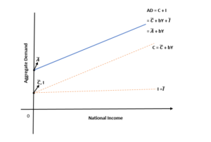
Important Concepts About Aggregate Demand
- Aggregate demand is a function of Consumption and investment only.
- The investment expenditure is assumed to be autonomous which means it will remain constant at all the levels of income.
- The investment curve will be a straight line, parallel to the X-axis as it is not affected by the change in income level.
- Consumption will be positive even at zero level of income as the minimum level of consumption is done for survival. This consumption is known as ‘Autonomous consumption’.
- The slope of the consumption curve is positive which shows that when income increases consumption also increases.
- The starting point of the AD curve is above zero as there is always a minimum level of consumption and investment in the economy.
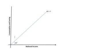
Meaning Of Aggregate Supply
Aggregate Supply is the value of all final goods and services that all the producers are planning to supply over a period of time.
Aggregate Supply =Y
HOW?: Output produced in an economy is always equal to the income generated. Aggregate Supply is equal to all final goods and services produced in the economy which is equal to the national income.
Aggregate Supply = OUTPUT =Y
Y = Aggregate Supply
Components Of Aggregate Supply
NATIONAL INCOME (Y) = CONSUMPTION (C) + SAVINGS (S)
Y = C + S
Consumption and savings are the two components of Aggregate Supply.
Aggregate Supply Schedule And Graph
Aggregate Supply = C + S
(i)Consumption(C)
(ii) Saving(S)
AS = C + S
| National Income (Y) | Consumption(C) | Saving (S) | AS = C + S |
| 0 | 20 | -20 | 0 |
| 10 | 25 | -15 | 10 |
| 20 | 30 | -10 | 20 |
| 30 | 35 | -5 | 30 |
| 40 | 40 | 0 | 40 |
| 50 | 45 | 5 | 50 |
| 60 | 50 | 10 | 60 |
Important Concept About Aggregate Supply
The slope of the AS curve is positive as the level of income increases aggregate supply also increases.
Consumption Function Or Propensity To Consume
Consumption function or propensity to consume is the functional relationship between consumption and income.
C= f (Y)
Consumption Schedule And Types Of Propensity To Consume
| Income(Y) | Consumption(C) | APC (C/Y) | ΔC | ΔY | MPC ( ΔC/ΔY) |
| 0 | 100 | – | – | – | – |
| 100 | 170 | 1.7 | 70 | 100 | 0.7 |
| 200 | 240 | 1.2 | 70 | 100 | 0.7 |
| 300 | 310 | 1.33 | 70 | 100 | 0.7 |
| 400 | 380 | 0.95 | 70 | 100 | 0.7 |
| 500 | 450 | 0.9 | 70 | 100 | 0.7 |
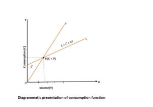
Important Points About Consumption
- The slope of the consumption curve is positive as consumption increases when leveling of income increases.
- The starting point of the consumption curve is above zero as the is always some minimum level of consumption which is termed as “Autonomous consumption”.
- The point where C=Y is termed as break-even point as at this point Consumption is equal to income.
- Before the break-even point in the economy because consumption is more than income after the break-even point savings will start as now the increase in consumption is less than the increase in income.
Types Of Propensity
-
- Average Propensity to Consume (APC)
- Marginal Propensity to) Consume (MPC)
Average Propensity To Consume(Apc)
APC is the ratio of total consumption to total income.
Average Propensity To Consume = C/Y
Important Concepts About Apc
- APC can never be zero as consumption can never be zero.
- At the break-even point, APC is equal to 1.
- Before the break-even point, APC is less than 1.
- After the break-even point, APC is more than 1.
- APC falls with an increase in income.
Marginal Propensity To Consume
MPC is the ratio of change in consumption to change in income.
MPC = ΔC / ΔY
Important Concepts About Mpc
- The value of MPC can never be greater than 1.
- The value of MPC is 1 when the entire additional income is spent on consumption
- The value of MPC is 0 when the entire additional income is saved.
- The value of MPC lies between 0 to 1.
Consumption Equation
C = c‾ + bY
Where
C= Level of consumption
C¯= Autonomous consumption
b = MPC
Y = Level of income
4th PPT
Savings Function Or Propensity To Save
Savings function or propensity to save is the functional relationship between savings and income.
S= f (Y)
Savings Schedule And Types Of Propensity To Save
| Income(Y) | Consumption(C) | Saving (S) | APS (S/Y | ΔS | ΔY | MPS (ΔS/ΔY ) |
| 0 | 100 | -100 | – | – | – | – |
| 100 | 160 | -60 | -0.6 | 40 | 100 | 0.4 |
| 200 | 220 | -20 | -0.1 | 40 | 100 | 0.4 |
| 300 | 280 | 20 | 0.067 | 40 | 100 | 0.4 |
| 400 | 340 | 60 | 0.15 | 40 | 100 | 0.4 |
| 500 | 400 | 100 | 0.2 | 40 | 100 | 0.4 |
| 600 | 460 | 140 | 0.233 | 40 | 100 | 0.4 |
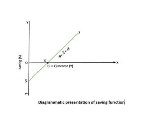
Important Points About Savings
- Savings Curve starts from origin.
- The slope of the savings curve is positive
- At the break-even point, savings are equals to 0.
- At the break-even point savings become positive.
Types Of Propensity To Save
- Average Propensity to Save (APS)
- Marginal Propensity to Save (MPS)
Average Propensity To Save(Aps)
APS is the ratio of total savings to total income.
APS = S/Y
Important Concepts About APS
- APS is zero at the break-even point.
- APS can never be equals to 1 or more than 1.
- APS can be negative or less than when.
Marginal Propensity To Save
MPS is the ratio of change in savings to change in savings.
MPS = ΔS / ΔY
Important Concepts About MPS
1. The value of MPS varies between 0 and 1.
- If the entire increased income is saved the value of MPS will be 1.
- If the entire increased income is consumed the value of MPS will be 0.
Savings Equation
S = – ¯c+ (1- b)Y
Where
C= Level of consumption
– ¯c= Negative savings at zero level of income
1-b = MPS
Y = Level of income
Relationship Between APC And APS
APC + APS = 1
Relationship Between MPC And MPS
MPC + MPS = 1
Full Employment And Involuntary Unemployment
FULL EMPLOYMENT: It is a situation when people who are willing and able to work are getting work.
Under full employment, there can be two types of unemployment
- Frictional Unemployment: Frictional unemployment can be defined as a type of unemployment that occurs when a person is in the process of moving from one job to another.
- Structural Unemployment: Structural unemployment occurs because of a mismatch between the skills workers have, and the jobs that are actually available in the market. Structural unemployment usually happens because of technological change.
Involuntary Unemployment
Involuntary unemployment refers to a situation when people are ready to work at the prevailing wage rate in the market but do not find a job.
CBSE Class 12 Economics Notes Term II Syllabus
Part A: Introductory Macroeconomics
- Circular Flow of Income Class 12 Notes
- Basic Concepts of Macroeconomics Class 12 Notes
- National Income and Related Aggregates Class 12 Notes – 10 Mark
- National Income and Related Aggregates Class 12 Numericals
- Determination of Income and Employment Class 12 Notes
- Aggregate Demand and Its Related Concepts Class 12 Notes
- Excess Demand and Deficit Demand Class 12 Notes
- National Income Determination and Investment Multiplier Class 12 Notes
Part B: Indian Economic Development
Current challenges facing Indian Economy – 12 Marks
Development Experience of India – A Comparison with Neighbours – 6 Marks